4. Power Sector Modeling

This section introduces the foundation of the Costa Rica Energy Analysis Model (CREAM). The model is designed to represent the national power system with a structure that balances technical accuracy and computational feasibility. It describes the system topology, including the regional division and interconnections, as well as the spatial and temporal resolution applied in the analysis. Key assumptions are documented to provide transparency in how generation technologies, demand patterns, and operational practices are represented. The section also outlines the treatment of critical operational parameters and the calibration process, ensuring that simulated results align with observed system performance.

The modeling framework is an energy system optimization model (ESOM), which provide a powerful approach to representing the long-term evolution of energy systems under a variety of technical, economic, and policy conditions. Compared to accounting or simulation-based tools, ESOMs offer greater capability to identify cost-effective pathways, resource allocation strategies, and system-level trade-offs. Nevertheless, their abstraction of operational details introduces limitations when representing short-term dynamics. The implementation follows a hybrid two-language design: the optimization core is developed in Julia, which offers significant speed advantages for solving large-scale linear problems, while tasks such as data preprocessing, visualization, and scenario management are handled in Python. The model is original, building on methodological insights from established frameworks such as OSeMOSYS and GENeSYS-MOD. Its design emphasizes computational performance making it suitable for experimental scenario analysis focused on Costa Rica’s energy transition, both in terms of mitigation and adaptation to climate change.

4.1 Model structure and caracterization

Costa Rica’s power system is characterized by high renewable penetration and a well-defined regional structure. Operationally, it is divided into three zones: Chorotega, Central, and Huetar-Brunca. The Chorotega region hosts the majority of national generation capacity, accounting for approximately 62%, while Central and Huetar-Brunca contribute 16% and 25%, respectively. On the demand side, consumption is highly concentrated in the Central region, which represents about 60% of total load, compared to roughly 20% in each of the other two zones. The generation mix relies heavily on hydropower, close to 70%, complemented by geothermal (about 20%), wind (10%), and minor contributions from solar and bagasse (<1%). This configuration yields an overall renewable share of around 98% in a typical year. However, in dry years—often linked to El Niño events—the renewable share can fall to about 89%, requiring thermal plants to supply the deficit. Transmission is arranged in a meshed, ring-like network with congestion issues on northern corridors, and international interconnections exist with Nicaragua and Panama, enabling transactions in the Central American market

As shown in Figure 4.1, the left panel shows the geographical division into three operational regions (Chorotega, Central, Huetar-Brunca). The right panel illustrates the network abstraction, where each node includes demand centers, existing generation capacity, and the potential integration of new technologies. Dashed lines represent candidate investments such as new plants, storage systems, or transmission reinforcements, while solid lines indicate existing interconnections, including international links with Nicaragua and Panama.

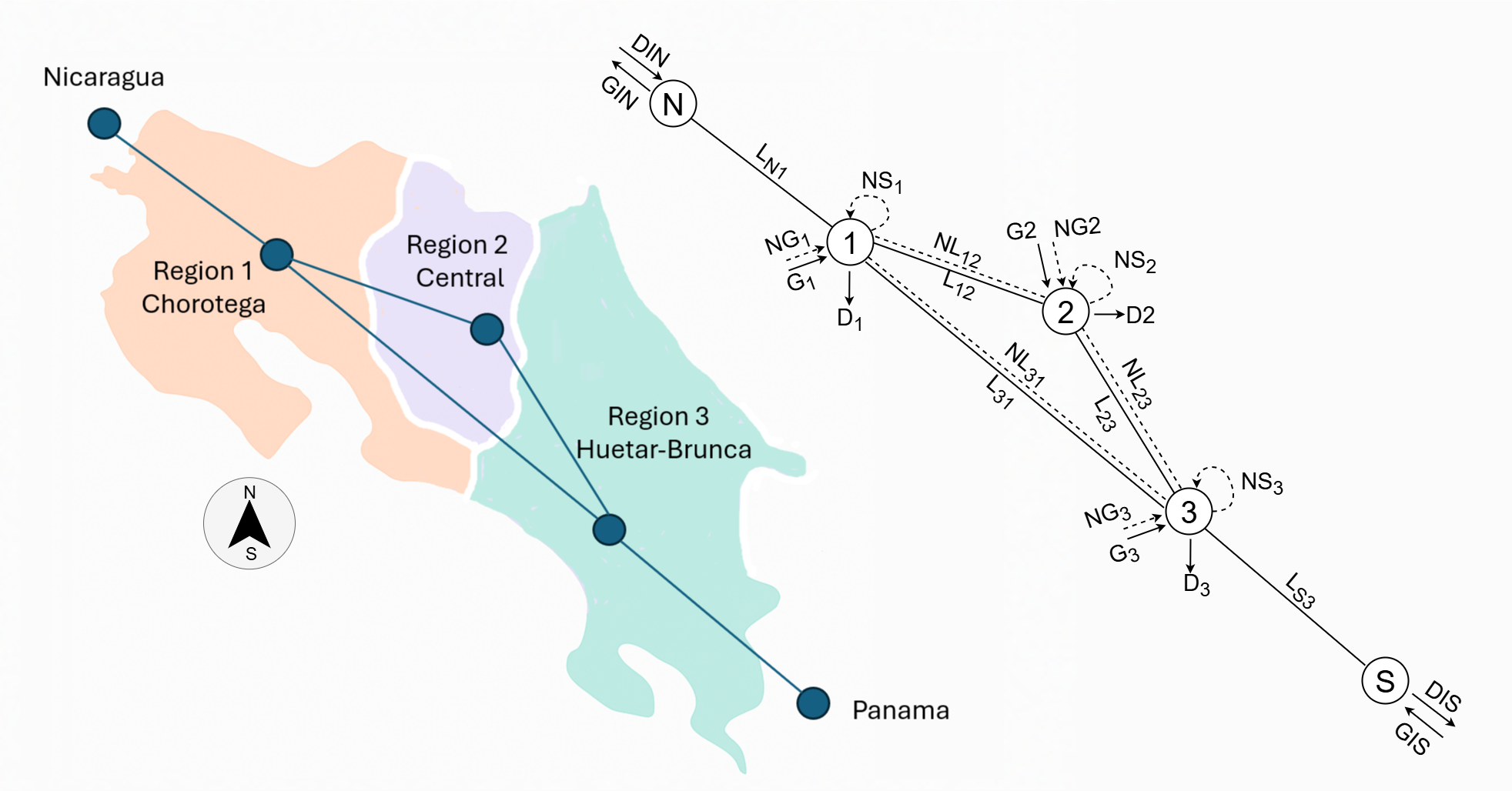
Figure 4.1. Geographical and graph-based representation of the Costa Rican power system

Figure 4.2 presents the node-level representation adopted in the model. Each node aggregates end-use demand modules—residential, commercial, and industrial baselines; decarbonization and digitalization levers; and separate light and heavy-duty EV charging, together with supply and flexibility assets. Generation technologies include geothermal, biomass, hydropower (reservoir and run-of-river), wind, solar, and thermal units. Batteries provide short-term storage, while transmission blocks represent interzonal and international links with bidirectional flows. The right-hand summary boxes list the key model sets (three regions, two seasons, forty-eight timeslices) and classify power plants by operational role (firm, flexible, variable, seasonal, backup). The modeling design aims to generate plausible scenarios, identify cost-effective investment portfolios across generation, storage, and transmission, and evaluate vulnerability and adaptation under climate change—particularly hydrologic stress in dry years and ENSO-driven variability. By coupling nodal structure with operational attributes and charging profiles, the framework captures system-level trade-offs among energy, flexibility, and curtailment, enabling transparent planning analyses.

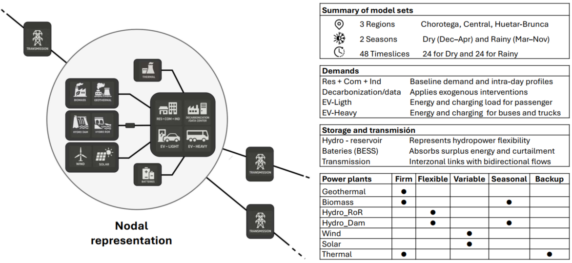
Figure 4.2. Node schematic: demand, generation, storage, transmission

4.3 Electricity Demand

Figure 4.3 presents the demand trajectories we are studying. Because the long term is inherently uncertain, we consider ranges of scenarios rather than single lines. The figure overlays historical trends with intervention curves tied to decarbonization policies, showing how policy-driven shifts can bend the baseline and widen the plausible envelope

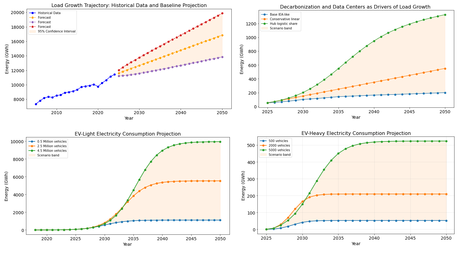
Figure 4.3. Demand Scenarios: Baseline, Decarbonization & Data Centers, EV-Light, EV-Heavy

Demand is a primary source of model uncertainty, and planning decisions should be assessed against the range of credible trajectories, not only the mean. Building on this principle, the baseline demand projection is derived from the national energy-balance time series, expressed in GWh. We estimate a univariate ARIMA model to capture the long-run trend and its stochastic variability, selecting orders via standard information criteria and validating residuals for whiteness and stability. The forecast (orange markers) is shown together with a 95% confidence interval (shaded band), which widens over the horizon as uncertainty accumulates. We interpret this band as an envelope of plausible baseline outcomes rather than a precise point estimate, using it to communicate both central tendency and dispersion. This baseline serves as a business-as-usual reference against which interventions are layered. In subsequent analyses, the baseline trajectories are systematically modified by scenario levers—such as decarbonization and data-center buildout—and by explicit electric-vehicle modules, enabling transparent stress testing of investment needs.

We include two families of interventions on the baseline: (i) economy-wide decarbonization and data-center buildout, and (ii) transport electrification. For decarbonization/data centers, we define parametric share trajectories (logistic, piecewise exponential, and linear) that map the fraction of total electricity attributable to these drivers; multiplying each share by the baseline yields annual GWh paths. Transport electrification is represented with separate light and heavy-duty modules. Each module uses a Bass-type diffusion for fleet adoption and converts stock into energy via per-vehicle assumptions (annual kilometers, kWh/km, charging efficiency).In all panels, shaded bands depict the scenario envelope—from conservative to high-uptake cases—capturing uncertainty around adoption speed, utilization, technology efficiency, and policy execution.

Figure 4.4 depicts the hourly demand profiles used in the model, expressed as per-unit of daily energy to allow shape comparisons across end uses. Each panel presents three representative profiles for a given demand class, with markers at hourly values and a shaded band showing the envelope between the minimum and maximum shapes. The Baseline panel contrasts a “Peak” profile with a pronounced evening ramp, a “Flat” profile with near-constant load, and a “Base” profile reflecting current diurnal variation. The Decarbonization & Data Centers panel represents additional industrial and data-center loads scheduled as “three shifts,” “two shifts,” and “round-the-clock,” allocating the same daily energy with different temporal concentrations depending on the industry class. EV-Light illustrates passenger EV charging strategies: “Smart Night” valley-filling, “Uncontrolled” arrival-driven evening charging, and a blended “Mean.” EV-Heavy captures fleet behavior: “Smart Night” depot charging, “Opportunity” daytime top-ups, and a balanced “Mean.” These shapes are paired with annual energy trajectories in scenario analysis to stress-test flexibility, storage, and transmission under alternative temporal patterns of emerging demand.

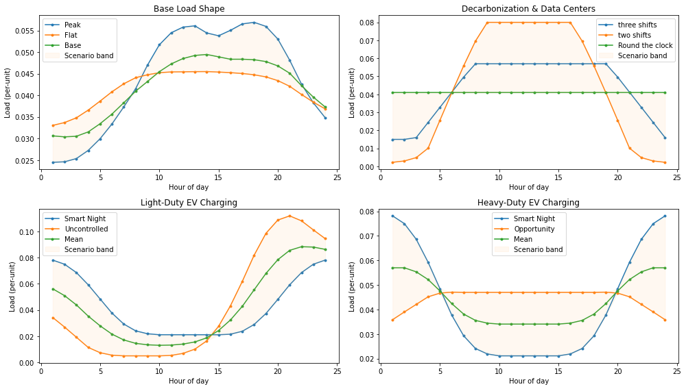
Figure 4.4. “Scenario Load Profiles: Baseline, Decarbonization & Data Centers, EV-Light, EV-Heavy

Figure 4.5 presents two complementary views: first, the baseline annual demand trajectory (business-as-usual) used as the reference for scenario perturbations; second, the hourly profiles employed for temporal allocation. In the profile panel, we include the base-year 2025 reference shape and a 2050 envelope that spans the range of plausible load shapes, from conservative to high-uptake cases. Together, these elements link long-run energy trajectories with diurnal load distribution for planning analysis. Working with envelopes rather than single lines enables robust comparison of investment needs across generation, storage, and transmission. These interventions are layered transparently on the baseline so attribution to each driver remains explicit and reproducible.

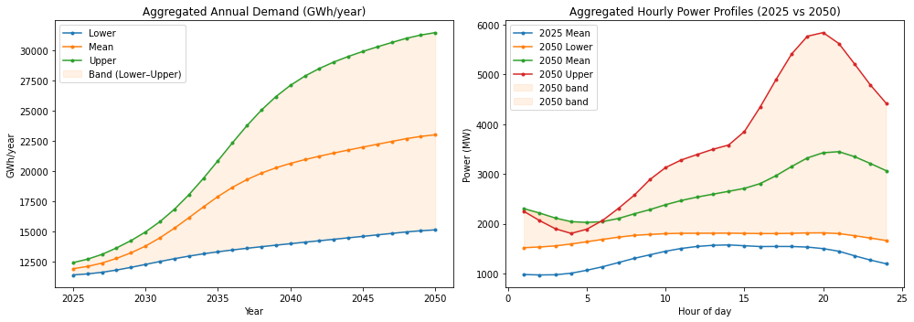
Figure 4.5. “Annual Demand Trajectory and Hourly Load Profiles for Costa Rica’s Electricity System

General equation:

Simple delays:

where ϕ corresponds to operators, μ is the media of ϕ, θ is a coefficient, and s is a stational component.

This forecasting model gives good approximations of the data registered by institutions. The estimation begins with the analysis and forecasting of the time series corresponding to the primary sources. With these long term values, a specific trend is fixed by using the shares defined in the base year. A Hierarchical process was develop considering that the shares by each sector are the same on the base year.

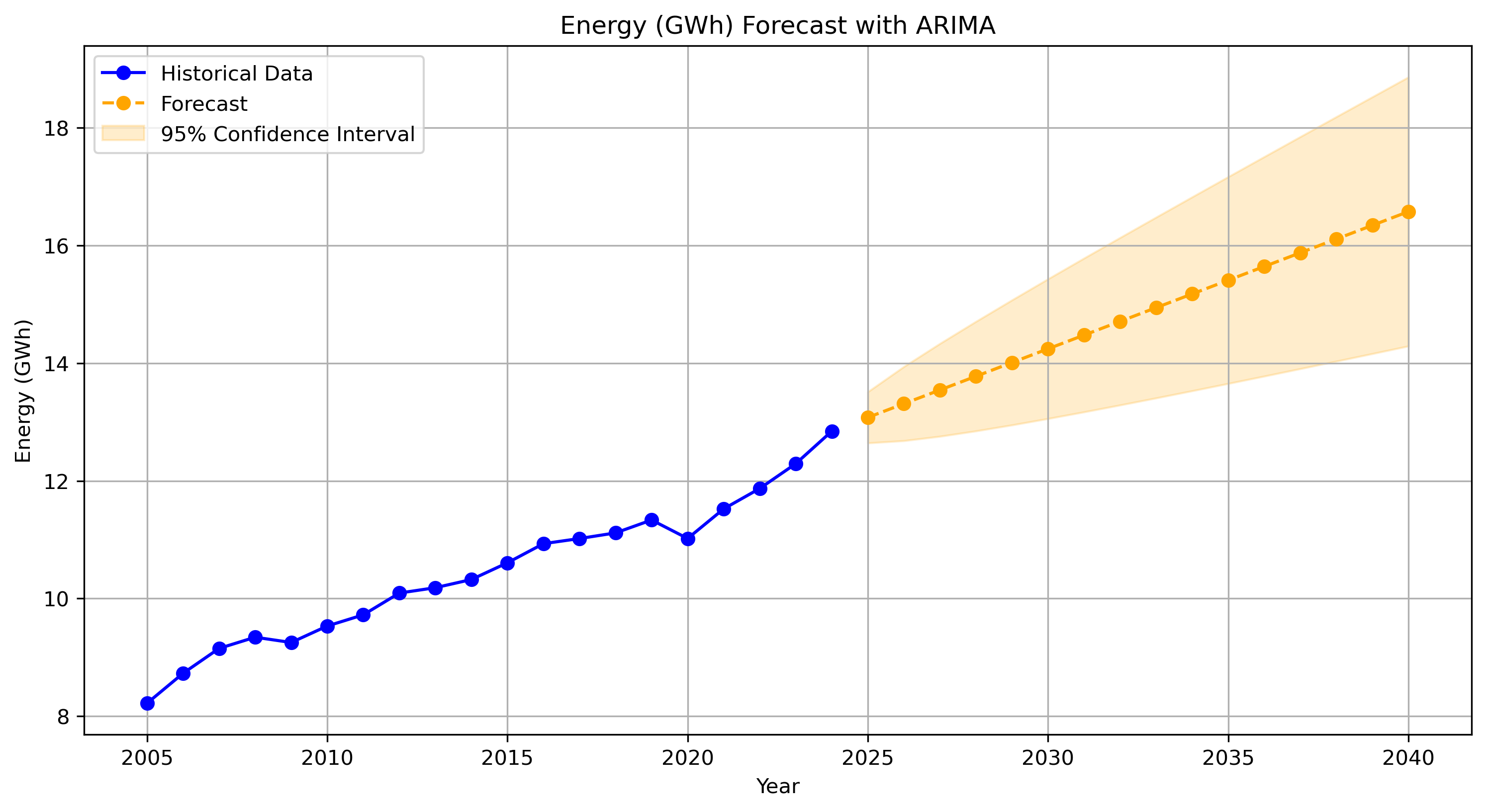
Figure 4.1: Historical and Forecasting electricity consumption by sector in Costa Rica

-Specified Annual Demand

-Specified Annual Demand

-Series intervention

4.4 Supply and performance

Capacity Factor Availability Factor Operational Life Residual Capacity Input Activity Ratio Output Activity Ratio

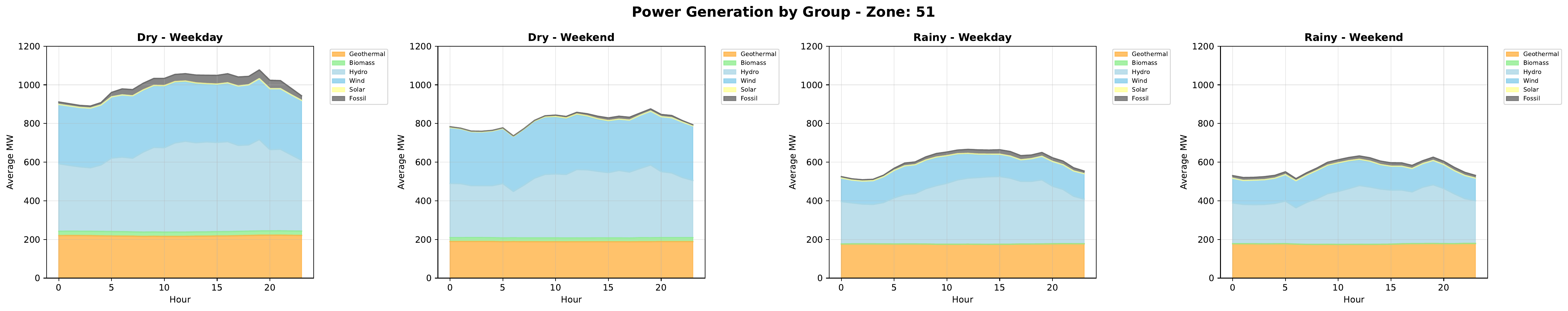
Figure XXX: Generation Region 1

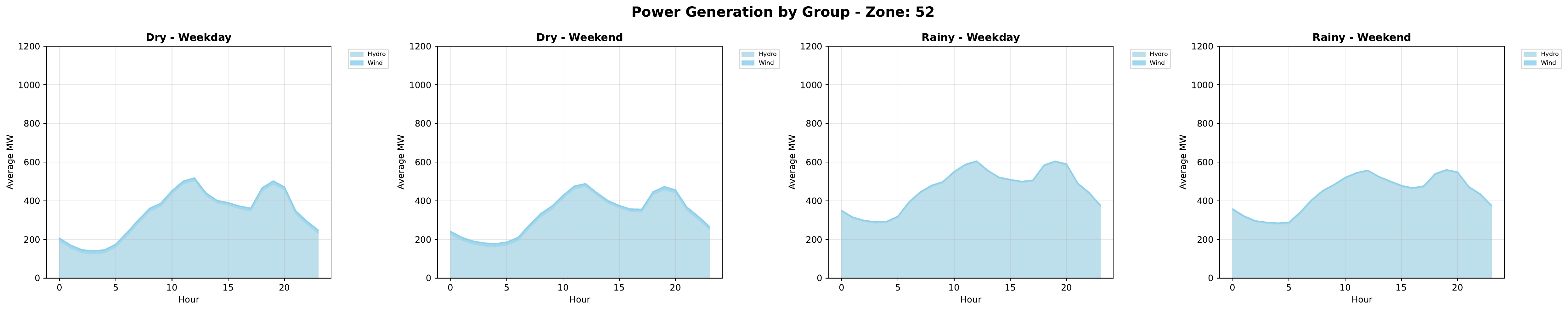
Figure XXX: Generation Region 2

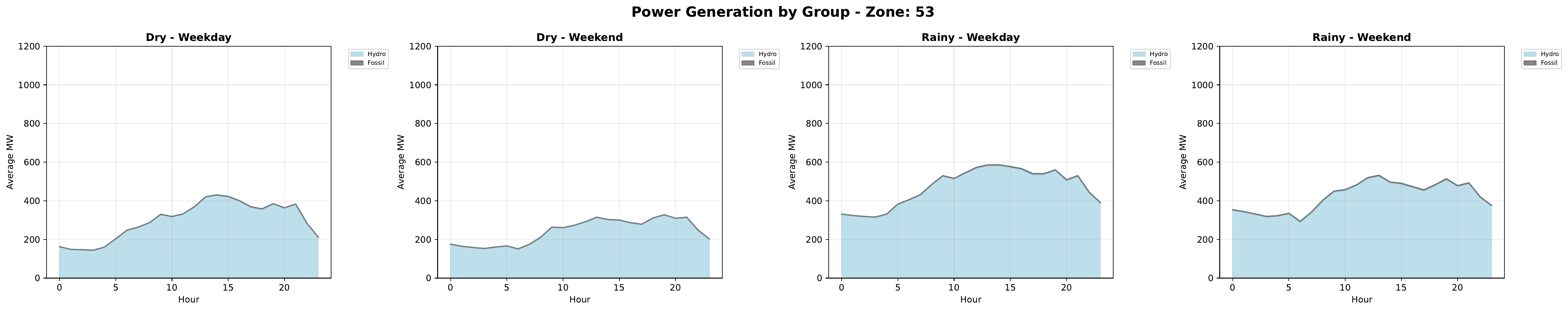
Figure XXX: Generation Region 3

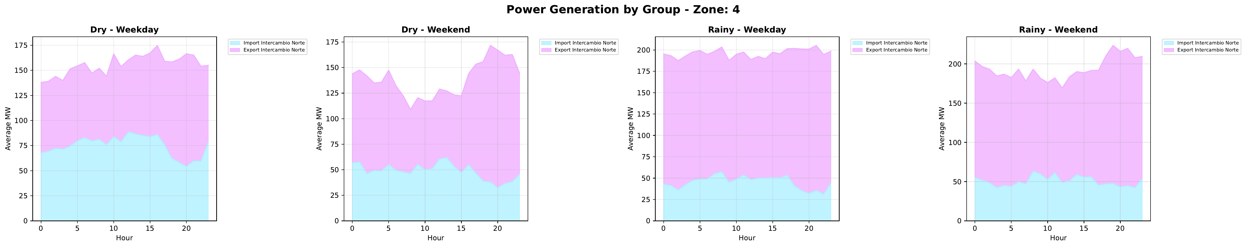
Figure XXX: Interchange Nicaragua

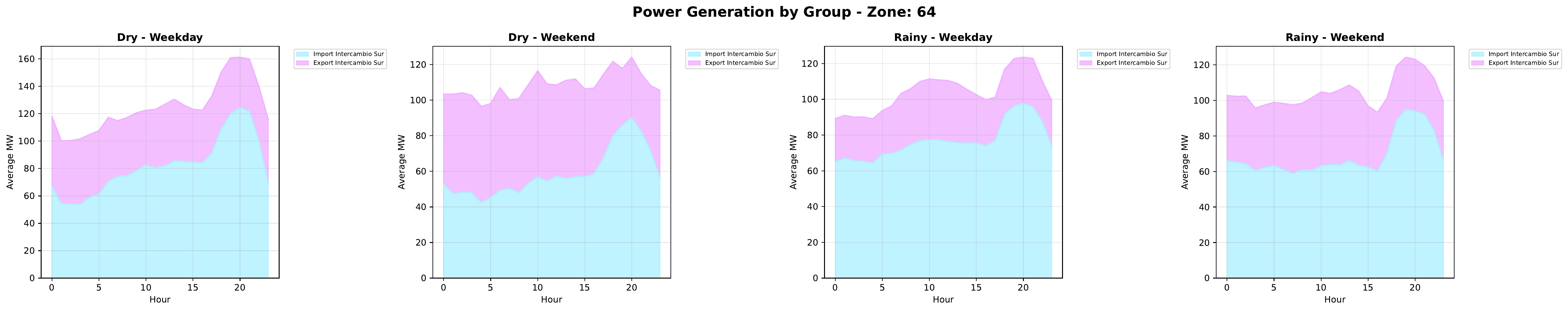
Figure XXX: Interchange Panama

Figure XXX: Generation National and Interchange

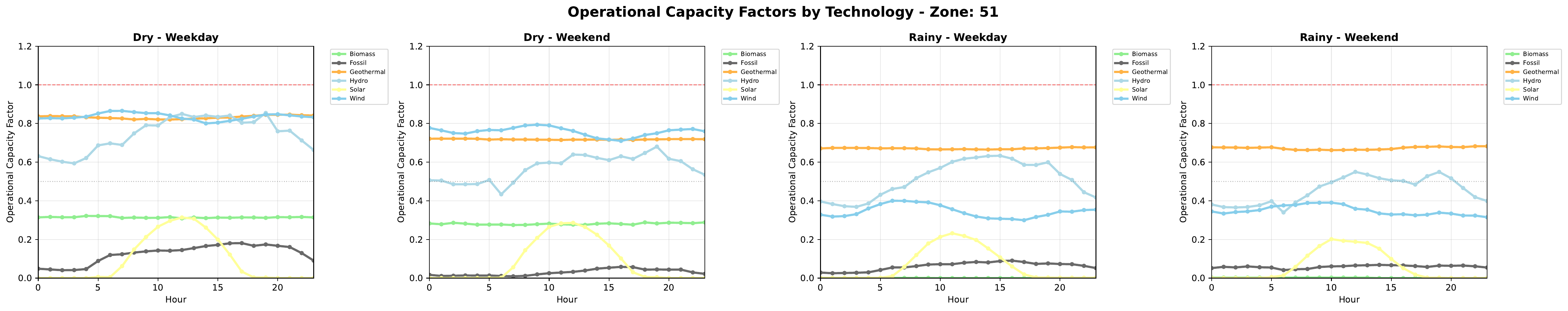
Figure XXX: Operational CF R1

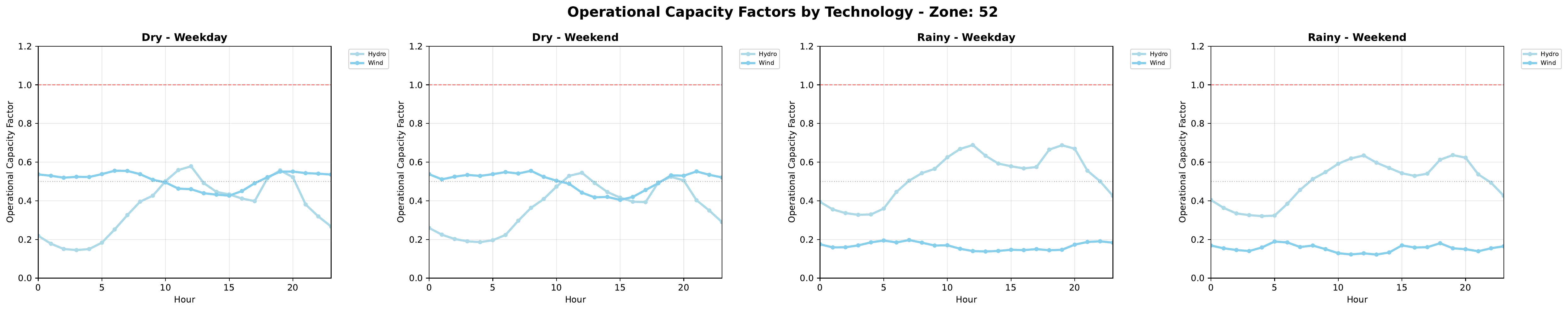
Figure XXX: OperationalCFR2

4.5 Technology costs

Capital and Fixed

4.6 Decision Parameters and Variables

CREAM Data & Model Specification

Scope & Resolution

• Regions: 5 (see data/set_regions.csv)

• Timeslices: 96 representative hourly slices per year (see Notes on timeslices)

• Planning years: 2025, 2030, 2035, 2040, 2045, 2050

• Final year treatment: snapshot (YDM[2050] = 1)

• Currency: constant USD2020

• Power unit: MW, Energy unit: MWh

Sets

Symbol	CSV	Description
	data/set_regions.csv	Regions (5 entries), column: region
	data/set_technologies.csv	Specially for power plants, column: technology
	data/set_fuels.csv	Power for electricity networks, column: fuel
	data/set_timeslices.csv	Representative hours, column: timeslice
	data/set_years.csv	Planning years (2025:5:2050), column: year
	data/storage_set_techs.csv	Storage technologies, column: storage
	data/trans_set_links.csv	Transmission links, columns: link_id, region_i, region_j

Year Weighting

YearlyDifferenceMultiplier (YDM)
- 2025,2030,2035,2040,2045 -> 5 (years represented by the node)
- 2050 -> 1 (snapshot)

Parameters (Data Dictionary)

Key: Indices shown as tuples of set symbols.

General power grid

Name	CSV	Sets	Units	Default	Notes / Source
AnnualEmissionLimit	param_emission_limit.csv	[Y]	tCO2/year	large	Policy cap per year.
EmissionRatio	param_activity_ratio_emission.csv	[T]	tCO2/MWh_out	0	Emission intensity per MWh output (single-fuel case).
InputActivityRatio	param_activity_ratio_input.csv	T,F	MWh_in per unit-activity	—	Maps activity to inputs (OSeMOSYS-style).
OutputActivityRatio	param_activity_ratio_output.csv	[T,F]	MWh_out per unit-activity	—	Maps activity to outputs (OSeMOSYS-style).
TagDispatchableTechnology	param_tag_dispatchable.csv	[T]	{0,1}	1	1=dispatchable; 0=VRE-like.
OperationalLife	param_lifetime.csv	[T]	years	—	Tech lifetime for cohort accounting & salvage.
AnnualDemand	param_demand_annual.csv	[Y,R,F]	MWh/year	—	Annual energy demand. Source: utility stats.
DemandProfile	param_demand_profile.csv	[R,H,F]	p.u. (sum_H=1)	1/|H|	Normalized hourly shape. One per (R,F). If omitted, uniform.
InvestmentCost	param_cost_investment.csv	[Y,T]	USD/MW_new	—	Overnight CAPEX.
FixedCost	param_cost_fixed.csv	[Y,T]	USD/(MW·year)	0	Fixed O&M per MW-year.
VariableCost	param_cost_variable.csv	[Y,T]	USD/MWh_out	—	Variable O&M on output basis.
CapacityFactor	param_capacity_factors.csv	[R,H,T]	p.u. [0–1]	—	Time-varying for VRE; for dispatchables can be flat.
MaxCapacity	param_capacity_max.csv	[Y,R,T]	MW	large	Siting/technical cap.
ResidualCapacity	param_capacity_residual.csv	[Y,R,T]	MW	0	Existing stock at year y.

Storage parameters

Name	CSV	Sets	Units	Default	Notes / Source
StorageInvestmentCost	storage_param_cost_investment.csv	(Y,S)	USD/MWh_energy_new	—	Energy capacity CAPEX.
StorageFixedCost	storage_param_cost_fixed.csv	(Y,S)	USD/(MWh·year)	0	Fixed O&M per MWh-year.
E2PRatio	storage_e2p_ratio.csv		hours	—	Energy-to-power ratio; Pmax = E/E2P.
StorageChargeEfficiency	storage_param_efficiency_charge.csv	(S,F)	p.u.	—	Charge efficiency.
StorageDischargeEfficiency	storage_param_efficiency_discharge.csv	(S,F)	p.u.	—	Discharge efficiency (>0 means storage is enabled for F).
StorageLosses	storage_param_losses.csv	(S,F)	p.u./timeslice	1.0	Retention per step (1 = no losses).
MaxStorageCapacity	storage_param_capacity_max.csv	(Y,R,S)	MWh	large	Upper bound on energy capacity.
StorageOperationalLife	storage_param_lifetime.csv		years	—	Lifetime for salvage & cohorting.

Transmission parameters

Name	CSV	Sets	Units	Default	Notes / Source
ResidualTransCap	trans_param_capacity_residual.csv	(Y,L)	MW	0	Existing interregional capacity.
MaxTransCap	trans_param_capacity_max.csv	(Y,L)	MW	large	Upper bound by corridor.
MinCapInvest	trans_param_capacity_min_investment.csv	(Y,L)	MW	0	Minimum lump size (enforces binary “build-or-not”).
InvCostTrans	trans_param_cost_investment.csv	(Y,L)	USD/MW_new	—	Line CAPEX per MW.
FixCostTrans	trans_param_cost_fixed.csv	(Y,L)	USD/(MW·year)	0	Annual O&M per MW.
LossFactorTrans	trans_param_losses.csv	(L,F)	p.u.	0	Fractional losses; efficiency .
TransLife	trans_param_lifetime.csv		years	—	Lifetime for salvage & cohorting.
DiscountRate	(code constant)	—	p.u./year	0.05	Social discount rate.
YearlyDifferenceMultiplier	(code-generated)		years	5 (2025..2045), 1 (2050)	Year weighting (block vs snapshot).

Variables

Name	Indices	Units	Interpretation
TotalCost	(Y,R,T)	USD	Tech total cost in year y (OPEX + Fixed·YDM + CAPEX).
FuelProductionByTechnology	(Y,R,H,T,F)	MWh	Output fuel from technology.
FuelUseByTechnology	(Y,R,H,T,F)	MWh	Input fuel to technology (linked via InputActivityRatio).
NewCapacity	(Y,R,T)	MW	Newly installed capacity.
AccumulatedCapacity	(Y,R,T)	MW	Installed capacity alive in year y (cohorted).
AnnualTechnologyEmissions	(Y,R,T)	tCO2	Annual emissions by tech and region.
Curtailment	(Y,R,H,F)	MWh	Unserved/curtailed fuel at node.
SalvageValue	(Y,R,T)	USD	Tech salvage (positive value; subtracted in objective).
NewStorageEnergyCapacity	(Y,R,S,F)	MWh	New storage energy capacity (enabled when discharge eff. > 0).
AccumulatedStorageEnergyCapacity	(Y,R,S,F)	MWh	Storage energy capacity alive in year y.
StorageCharge / StorageDischarge	(Y,R,S,H,F)	MWh	Charge and discharge energy flows.
StorageLevel	(Y,R,S,H,F)	MWh	State of charge.
TotalStorageCost	(Y,R,S)	USD	Storage cost (CAPEX + Fixed·YDM).
StorageSalvageValue	(Y,R,S)	USD	Storage salvage (subtracted in objective).
NewTransCap	(Y,L)	MW	New transmission capacity.
AccumTransCap	(Y,L)	MW	Transmission capacity alive in year y.
FlowPlus / FlowMinus	(Y,H,L,F)	MWh	Directed flows (i→j) and (j→i).
TotalTransmissionCost	(Y,L)	USD	Transmission cost (CAPEX + Fixed·YDM).
TransmissionSalvageValue	(Y,L)	USD	Transmission salvage (subtracted in objective).
BuildTrans	(Y,L)	{0,1}	Binary “build-or-not” for minimum lump size.

Notes on Timeslices

• 96 slices represent typical weekly/seasonal and diurnal variation.

• Demand profiles are normalized per (R,F) so that .

• If using capacity factors for VRE, ensure their averaging matches the timeslice construction.

File Layout

docs/
  data/
    set_regions.csv
    set_technologies.csv
    set_fuels.csv
    storage_set_techs.csv
    trans_set_links.csv
    param_*.csv
    storage_*.csv
    trans_*.csv
_static/
  capacity_factors.png
index.rst
model_spec.rst   <-- (this file)